Ariely.nbThe “Ariely” fake result reveal a probability distribution totally foreign to psychologists
Ariely.nbThe “Ariely” fake result reveal a probability distribution totally foreign to psychologists
From @infseriesbot, prove the identity: \(\gamma_n = \displaystyle\int_1^\infty \frac{\{x\}}{x^2} (n-\log(x)) \log^{n-1} \, dx \).
We have \(\{x\}=x-i \, \text{for} \, i \leq x \leq i+1\),
so
\(\text{rhs}=\displaystyle\sum _{i=1}^{\infty } \displaystyle\int_i^{i+1} \frac{(x-i) (n-\log (x)) \log ^{n-1}(x)}{x^2} \, dx,\)
and since \(\displaystyle\int \frac{(x-i) (n-x \log ) \left(x \log ^{n-1}\right)}{x^2} \, dx=\log ^n(x) \left(-\frac{i}{x}-\frac{\log (x)}{n+1}+1\right)\)
\(\displaystyle \int_i^{i+1} \frac{(x-i) (n-\log (x)) \log ^{n-1}(x)}{x^2} \, dx=\frac{(i+1) \log ^{n+1}(i)+(-(i+1) \log (i+1)+n+1) \log ^n(i+1)}{(i+1) (n+1)}\),
allora:
\(\text{rhs}=\underset{T\to \infty }{\text{lim}}\left(\frac{(n-(T+1) \log (T+1)+1) \log ^n(T+1)}{(n+1) (T+1)}+\sum _{i=2}^T \frac{\log ^n(i)}{i}\right)\),
and since \(\frac{\log ^n(T+1) (n-(T+1) \log (T+1)+1)}{(n+1) (T+1)}\overset{T}{\to}\frac{\log ^{n+1}(T)}{n+1}\),
From the series representation of the Stieltjes Gamma function, \(\gamma_n\):
\(\underset{T\to \infty }{\text{lim}}\left(\sum _{i=1}^T \frac{\log ^n i}{i}-\frac{\log ^{n+1}(T)}{n+1}\right)=\gamma _n\)
You have zero probability of making money. But it is a great trade.
One-tailed distributions entangle scale and skewness. When you increase the scale, their asymmetry pushes the mass to the right rather than bulge it in the middle. They also illustrate the difference between probability and expectation as well as the difference between various modes of convergence.
Consider a lognormal \(\mathcal{LN}\) with the following parametrization, \(\mathcal{LN}\left[\mu t-\frac{\sigma ^2 t}{2},\sigma \sqrt{t}\right]\) corresponding to the CDF \(F(K)=\frac{1}{2} \text{erfc}\left(\frac{-\log (K)+\mu t-\frac{\sigma ^2 t}{2}}{\sqrt{2} \sigma \sqrt{t}}\right) \).
The mean \(m= e^{\mu t}\), does not include the parameter \(\sigma\) thanks to the \(-\frac{\sigma ^2}{2} t\) adjustment in the first parameter. But the standard deviation does, as \(STD=e^{\mu t} \sqrt{e^{\sigma ^2 t}-1}\).
When \(\sigma\) goes to \(\infty\), the probability of exceeding any positive \(K\) goes to 0 while the expectation remains invariant. It is because it masses like a Dirac stick at \(0\) with an infinitesimal mass at infinity which gives it a constant expectation. For the lognormal belongs to the log-location-scale family.
\(\underset{\sigma \to \infty }{\text{lim}} F(K)= 1\)
Option traders experience an even worse paradox, see my Dynamic Hedging. As the volatility increases, the delta of the call goes to 1 while the probability of exceeding the strike, any strike, goes to \(0\).
More generally, a \(\mathcal{LN}[a,b]\) has for mean, STD, and CDF \(e^{a+\frac{b^2}{2}},\sqrt{e^{b^2}-1} e^{a+\frac{b^2}{2}},\frac{1}{2} \text{erfc}\left(\frac{a-\log (K)}{\sqrt{2} b}\right)\) respectively. We can find a parametrization producing weird behavior in time as \(t \to \infty\).
Thanks: Micah Warren who presented a similar paradox on Twitter.
The main paper Bitcoin, Currencies and Fragility is updated here .
The supplementary material is updated here
www.fooledbyrandomness.com/BTC-QF-appendix.pdf
BTC-QF-appendix
Prove
\(I= \displaystyle\int_{-\infty }^{\infty}\sum_{n=0}^{\infty } \frac{\left(-x^2\right)^n }{n!^{2 s}}\; \mathrm{d}x= \pi^{1-s}\).
We can start as follows, by transforming it into a generalized hypergeometric function:
\(I=\displaystyle\int_{-\infty }^{\infty }\, _0F_{2 s-1} (\overbrace{1,1,1,…,1}^{2 s-1 \text{times}}; -x^2)\mathrm{d}x\), since, from the series expansion of the generalized hypergeometric function, \(\, _pF_q\left(a_1,a_p;b_1,b_q;z\right)=\sum_{k=0}^{\infty } \frac{\prod_{j=1}^p \left(a_j\right)_k z^k}{\prod_{j=1}^q k! \left(b_j\right)_k}\), where \((.)_k\) is the Pochhammer symbol \((a)_k=\frac{\Gamma (a+k)}{\Gamma (a)}\).
Now the integrand function does not appear to be convergent numerically, except for \(s= \frac{1}{2}\) where it becomes the Gaussian integral, and the case of \(s=1\) where it becomes a Bessel function. For \(s=\frac{3}{2}\) and \( x=10^{19}\), the integrand takes values of \(10^{1015852872356}\) (serious). Beyond that the computer starts to produce smoke. Yet it eventually converges as there is a closed form solution. It is like saying that it works in theory but not in practice!

For, it turns out, under the restriction that \(2 s\in \mathbb{Z}_{>\, 0}\), we can use the following result:
\(\int_0^{\infty } t^{\alpha -1} _pF_q \left(a_1,\ldots ,a_p;b_1,\ldots ,b_q;-t\right) \, dt=\frac{\Gamma (\alpha ) \prod {k=1}^p \Gamma \left(a_k-\alpha \right)}{\left(\prod {k=1}^p \Gamma \left(a_k\right)\right) \prod {k=1}^q \Gamma \left(b_k-\alpha \right)}\)
Allora, we can substitute \(x=\sqrt(u)\), and with \(\alpha =\frac{1}{2},p=0,b_k=1,q=2 s-1\), given that \(\Gamma(\frac{1}{2})=\sqrt(\pi)\),
\(I=\frac{\sqrt{\pi }}{\prod _{k=1}^{2 s-1} \sqrt{\pi }}=\pi ^{1-s}\).
So either the integrand eventually converges, or I am doing something wrong, or both. Perhaps neither.
Background: We’ve discussed blood pressure recently with the error of mistaking the average ratio of systolic over diastolic for the ratio of the average of systolic over diastolic. I thought that a natural distribution would be the gamma and cousins, but, using the Framingham data, it turns out that the lognormal works better. For one-tailed distribution, we do not have a lot of choise in handling higher dimensional vectors. There is some literature on the multivariate gamma but it is neither computationally convenient nor a particular good fit.
Well, it turns out that the Lognormal has some powerful properties. I’ve shown in a paper (now a chapter in The Statistical Consequences of Fat Tails) that, under some parametrization (high variance), it can be nearly as “fat-tailed” as the Cauchy. And, under low variance, it can be as tame as the Gaussian. These academic disputes on whether the data is lognormally or power law distributed are totally useless. Here we realize that by using the method of dual distribution, explained below, we can handle matrices rather easily. Simply, if \(Y_1, Y_2, \ldots Y_n\) are jointly lognormally distributed with a covariance matrix \(\Sigma_L\), then \(\log(Y_1), \log(Y_2), \ldots \log(Y_n)\) are normally distributed with a matrix \(\Sigma_N\). As to the transformation \(\Sigma_L \to \Sigma_N\), we will see the operation below.
Let \(X_1=x_{1,1},\ldots,x_{1,n}, X_2= x_{2,1},\dots x_{2,n}\) be joint distributed lognormal variables with means \(\left(e^{\mu _1+\frac{\sigma _1^2}{2}}, e^{\mu _2+\frac{\sigma _2^2}{2}}\right)\) and a covariance matrix
\(\Sigma_L=\left(\begin{array}{cc}\left(e^{\sigma _1^2}-1\right) e^{2 \mu _1+\sigma _1^2}&e^{\mu _1+\mu _2+\frac{\sigma _1^2}{2}+\frac{\sigma _2^2}{2}}\left(e^{\rho \sigma _1 \sigma _2}-1\right)\\ e^{\mu _1+\mu _2+\frac{\sigma _1^2}{2}+\frac{\sigma _2^2}{2}}\left(e^{\rho \sigma _1 \sigma _2}-1\right)&\left(e^{\sigma _2^2}-1\right) e^{2 \mu _2+\sigma _2^2}\end{array}\right)\)
allora \(\log(x_{1,1}),\ldots, \log(x_{1,n}), \log(x_{2,1}),\dots \log(x_{2,n})\) follow a normal distribution with means \((\mu_1, \mu_2)\) and covariance matrix
\(\Sigma_N=\left(\begin{array}{cc}\sigma _1^2&\rho \sigma _1 \sigma _2 \\ \rho \sigma _1 \sigma _2&\sigma _2^2 \\ \end{array}\right)\)
So we can fit one from the other. The pdf for the joint distribution for the lognormal variables becomes:

\(f(x_1,x_2)= \frac{\exp \left(\frac{-2 \rho \sigma _2 \sigma _1 \left(\log \left(x_1\right)-\mu _1\right) \left(\log \left(x_2\right)-\mu _2\right)+\sigma _1^2 \left(\log \left(x_2\right)-\mu _2\right){}^2+\sigma _2^2 \left(\log \left(x_1\right)-\mu _1\right){}^2}{2 \left(\rho ^2-1\right) \sigma _1^2 \sigma _2^2}\right)}{2 \pi x_1 x_2 \sqrt{-\left(\left(\rho ^2-1\right) \sigma _1^2 \sigma _2^2\right)}}\)
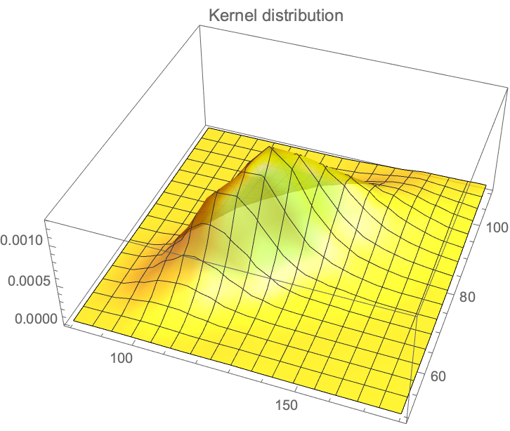
We have the data from the Framingham database for, using \(X_1\) for the systolic and \(X_2\) for the diastolic, with \(n=4040, Y_1= \log(X_1), Y_2=\log(X_2): {\mu_1=4.87,\mu_2=4.40, \sigma_1=0.1575, \sigma_2=0.141, \rho= 0.7814}\), which maps to: \({m_1=132.35, m_2= 82.89, s_1= 22.03, s_2=11.91}\).
The Lancet article: Maron, Barry J., and Paul D. Thompson. “Longevity in elite athletes: the first 4-min milers.” The Lancet 392, no. 10151 (2018): 913 contains an eggregious probabilistic mistake in handling “expectancy” a severely misunderstood –albeit basic– mathematical operator. It is the same mistake you read in the journalistic “evidence based” literature about ancient people having short lives (discussed in Fooled by Randomness), that they had a life expectancy (LE) of 40 years in the past and that we moderns are so much better thanks to cholesterol lowering pills. Something elementary: unconditional life expectancy at birth includes all people who are born. If only half die at birth, and the rest live 80 years, LE will be ~40 years. Now recompute with the assumption that 75% of children did not make it to their first decade and you will see that life expectancy is a statement of, mostly, child mortality. It is front-loaded. As child mortality has decreased in the last few decades, it is less front-loaded but it is cohort-significant.
The article (see the Table below) compares the life expectancy of athletes in a healthy cohort of healthy adults to the LE at birth of the country of origin. Their aim was to debunk the theory that while exercise is good, there is a nonlinear dose-response and extreme exercise backfires.

Something even more elementary missed in the Lancet article. If you are a nonsmoker, healthy enough to run a mile (at any speed), do not engage in mafia activities, do not do drugs, do not have metabolic syndrome, do not do amateur aviation, do not ride a motorcycle, do not engage in pro-Trump rioting on Capitol Hill, etc., then unconditional LE has nothing to do with you. Practically nothing.
Just consider that 17% of males today smoke (and perhaps twice as much at the time of the events in the “Date” column of the table). Smoking reduces your life expectancy by about 10 years. Also consider that a quarter or so of Americans over 18 and more than half of those over 50 have metabolic syndrome (depending on how it is defined).
Now some math. What is the behavior of life expectancy over time?
Let \(X\) be a random variable that lives in \((0,\infty)\) and \(\mathbb{E}\) the expectation operator under “real world” (physical) distribution. By classical results, see the exact exposition in The Statistical Consequences of Fat Tails:
\(\lim_{K \to \infty} \frac{1}{K} \mathbb{E}(X|_{X>K})= \lambda\)
If \(\lambda=1\) , \(X\) is said to be in the thin tailed class \(\mathcal{D}_1\) and has a characteristic scale . It means life expectancy decreases with age, owing to senescence, or, more rigorously, an increase of the force of mortality/hazard rate over time.
If \(\lambda>1\) , \(X\) is said to be in the fat tailed regular variation class \(\mathcal{D}2\) and has no characteristic scale. This is the Lindy effect where life expectancy increases with age.
If \(\lim_{K \to \infty} \mathbb{E}(X|_{X>K})-K= \lambda\) where \(\lambda >0\), then \(X\) is in the borderline exponential class.
The next conversation will be about the controversy as to whether human centenarians, after aging is done, enter the third class, just like crocodiles observed in the wild, where LE is a flat number (but short) regardless of age. It may be around 2 years whether one is 100 or 120.
In Yalta, K., Ozturk, S., & Yetkin, E. (2016). “Golden Ratio and the heart: A review of divine aesthetics”,
In Yalta, K., Ozturk, S., & Yetkin, E. (2016). “Golden Ratio and the heart: A review of divine aesthetics”,
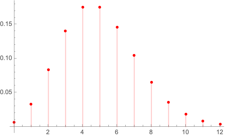
The Danish Mask Study presents the interesting probability problem: the odds of getting 5 infections for a group of 2470, vs 0 for one of 2398. It warrants its own test statistic which allows us to look at all conditional probabilities. Given that we are dealing with tail probabilities, normal approximations are totally out of order. Further we have no idea from the outset on whether the sample size is sufficient to draw conclusions from such a discrepancy (it is).
There appears to be no exact distribution in the literatrue for \(Y=X_ 1-X_2\) when both \(X_1\) and \(X_2\) are binomially distributed with different probabilities. Let’s derive it.
Let \(X_1 \sim \mathcal{B}\left(n_1,p_1\right)\), \(X_2 \sim \mathcal{B}\left(n_2,p_2\right)\), both independent.
We have the constrained probability mass for the joint \(\mathbb{P}\left(X_1=x_1,X_2=x_2\right)=f\left(x_2,x_1\right)\):
\(f\left(x_2,x_1\right)= p_1^{x_1} p_2^{x_2} \binom{n_1}{x_1} \binom{n_2}{x_2} \left(1-p_1\right){}^{n_1-x_1} \left(1-p_2\right){}^{n_2-x_2} \),
$latex x_1\geq 0\land n_1-x_1\geq 0\land x_2\geq 0\land n_2-x_2\geq 0 \$,
with \(x_1\geq 0\land n_1-x_1\geq 0\land x_2\geq 0\land n_2-x_2\geq 0\).
For each “state” in the lattice, we need to sum up he ways we can get a given total times the probability, which depends on the number of partitions. For instance:
Condition for \(Y \geq 0\) :
\(\mathbb{P} (Y=0)=f(0,0)=\)
\(\mathbb{P} (Y=1)=f(1,0)+f(2,1) \ldots +f\left(n_1,n_1-1\right)\),
so
\(\mathbb{P} (Y=y)=\sum _{k=y}^{n_1} f(k,k-y)\).
Condition for \(Y < 0\):
\(\mathbb{P} (Y=-1)=f(0,1)+f(1,2)+\ldots +\left(n_2-1,n_2\right)\),
alora
\(\mathbb{P} (Y=y)\sum _{k=y}^{n_2-y} f(k,k-y)\) (unless I got mixed up with the symbols).

The characteristic function:
\(\varphi(t)= \left(1+p_1 \left(-1+e^{i t}\right)\right){}^{n_1} \left(1+p_2 \left(-1+e^{-i t}\right)\right){}^{n_2}\)
Allora, the expectation: \(\mathcal{E}(Y)= n_1 p_1-n_2 p_2\)
The variance: \(\mathcal{V}(Y)= n_1^2 p_1^2 \left(\left(\frac{1}{1-p_1}\right){}^{n_1}\left(1-p_1\right){}^{n_1}-1\right)-n_1 p_1 \left(\left(\frac{1}{1-p_1}\right){}^{n_1}\left(1-p_1\right){}^{n_1}+p_1 \left(\frac{1}{1-p_1}\right){}^{n_1}\left(1-p_1\right){}^{n_1}+2 n_2 p_2 \left(\left(\frac{1}{1-p_1}\right){}^{n_1}\left(1-p_1\right){}^{n_1} \left(\frac{1}{1-p_2}\right){}^{n_2}\left(1-p_2\right){}^{n_2}-1\right)\right)-n_2 p_2 \left(n_2 p_2\left(\left(\frac{1}{1-p_2}\right){}^{n_2}\left(1-p_2\right){}^{n_2}-1\right)-\left(\frac{1}{1-p_2}\right){}^{n_2}\left(1-p_2\right){}^{n_2+1}\right)\)
The kurtosis:
\(\mathcal{K}=\frac{n_1 p_1 \left(1-p_1\right){}^{n_1-1} \, _4F_3\left(2,2,2,1-n_1;1,1,1;\frac{p_1}{p_1-1}\right)-\frac{n_2 p_2 \left(\left(1-p_2\right){}^{n_2} \, _4F_3\left(2,2,2,1-n_2;1,1,1;\frac{p_2}{p_2-1}\right)+n_2 \left(p_2-1\right) p_2 \left(\left(n_2^2-6 n_2+8\right) p_2^2+6 \left(n_2-2\right) p_2+4\right)\right)+n_1^4 \left(p_2-1\right) p_1^4-6 n_1^3 \left(1-p_1\right) \left(1-p_2\right) p_1^3-4 n_1^2 \left(2 p_1^2-3 p_1+1\right) \left(1-p_2\right) p_1^2+6 n_1 n_2 \left(1-p_1\right) \left(1-p_2\right){}^2 p_2 p_1}{p_2-1}}{\left(n_1^2 p_1^2 \left(\left(\frac{1}{1-p_1}\right){}^{n_1} \left(1-p_1\right){}^{n_1}-1\right)-n_1 p_1 \left(-\left(\frac{1}{1-p_1}\right){}^{n_1} \left(1-p_1\right){}^{n_1}+p_1 \left(\frac{1}{1-p_1}\right){}^{n_1} \left(1-p_1\right){}^{n_1}+2 n_2 p_2 \left(\left(\frac{1}{1-p_1}\right){}^{n_1} \left(1-p_1\right){}^{n_1} \left(\frac{1}{1-p_2}\right){}^{n_2} \left(1-p_2\right){}^{n_2}-1\right)\right)-n_2 p_2 \left(n_2 p_2 \left(\left(\frac{1}{1-p_2}\right){}^{n_2} \left(1-p_2\right){}^{n_2}-1\right)-\left(\frac{1}{1-p_2}\right){}^{n_2} \left(1-p_2\right){}^{n_2+1}\right)\right){}^2} \)
Every study needs its own statistical tools, adapted to the specific problem, which is why it is a good practice to require that statisticians come from mathematical probability rather than some software-cookbook school. When one uses canned software statistics adapted to regular medicine (say, cardiology), one is bound to make severe mistakes when it comes to epidemiological problems in the tails or ones where there is a measurement error. The authors of the study discussed below (The Danish Mask Study) both missed the effect of false positive noise on sample size and a central statistical signal from a divergence in PCR results. A correct computation of the odds ratio shows a massive risk reduction coming from masks.
The article by Bundgaard et al., [“Effectiveness of Adding a Mask Recommendation to Other Public Health Measures to Prevent SARS-CoV-2 Infection in Danish Mask Wearers”, Annals of Internal Medicine (henceforth the “Danish Mask Study”)] relies on the standard methods of randomized control trials to establish the difference between the rate of infections of people wearing masks outside the house v.s. those who don’t (the control group), everything else maintained constant.
The authors claimed that they calibrated their sample size to compute a p-value (alas) off a base rate of 2% infection in the general population.
The result is a small difference in the rate of infection in favor of masks (2.1% vs 1.8%, or 42/2392 vs. 53/2470), deemed by the authors as not sufficient to warrant a conclusion about the effectiveness of masks.
We would like to alert the scientific community to the following :

Immediate result: the study is highly underpowered –except ironically for the PCR and PCR+clinical results that are overwhelming in evidence.
Further: