
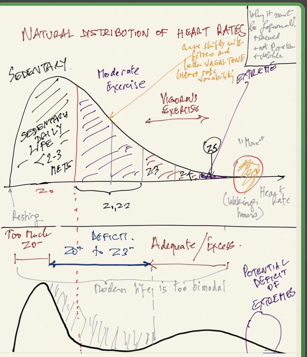
Heart rates must be Lognormal in distribution. Simply, it is not possible to have a negative heart rate and at low variance (and a mean > 6 standard deviations away from 0), the lognormal behaves like a normal.
Incidentally I failed
Heart rates must be Lognormal in distribution. Simply, it is not possible to have a negative heart rate and at low variance (and a mean > 6 standard deviations away from 0), the lognormal behaves like a normal.
Incidentally I failed

Financial theory requires correlation to be constant (or, at least, known and nonrandom). Nonrandom means predictable with waning sampling error over the period concerned. Ellipticality is a condition more necessary than thin tails, recall my Twitter fight with that non-probabilist Clifford Asness where I questioned not just his empirical claims and his real-life record, but his own theoretical rigor and the use by that idiot Antti Ilmanen of cartoon models to prove a point about tail hedging. Their entire business reposes on that ghost model of correlation-diversification from modern portfolio theory. The fight was interesting sociologically, but not technically. What is interesting technically is the thingy below.
How do we extract sampling error of a rolling correlation? My coauthor and I could not find it in the literature so we derive the test statistics. The result: it has less than \(10^{-17}\) odds of being sampling error.
The derivations are as follows:
Let \(X\) and \(Y\) be \(n\) independent Gaussian variables centered to a mean \(0\). Let \(\rho_n(.)\) be the operator.
\(\rho_n(\tau)= \frac{X_\tau Y_\tau+X_{\tau+1} Y_{\tau+1}\ldots +X_{\tau+n-1} Y_{\tau+n-1}}{\sqrt{(X_{\tau}^2+X_{\tau+1}^2\ldots +X_{\tau+n-1}^2)(Y_\tau^2+Y_{\tau+1}^2\ldots +Y_{\tau+n-1}^2)}}.\)\
First, we consider the distribution of the Pearson correlation for \(n\) observations of pairs assuming \(\mathbb{E}(\rho) \approx 0\) (the mean is of no relevance as we are focusing on the second moment):
\(f_n(\rho)=\frac{\left(1-\rho^2\right)^{\frac{n-4}{2}}}{B\left(\frac{1}{2},\frac{n-2}{2}\right)},\)
with characteristic function:
\(\chi_n(\omega)=2^{\frac{n-1}{2}-1} \omega ^{\frac{3-n}{2}} \Gamma \left(\frac{n}{2}-\frac{1}{2}\right) J_{\frac{n-3}{2}}(\omega ),\)
where \(J_{(.)}(.)\) is the Bessel J function.
We can assert that, for \(n\) sufficiently large: \(2^{\frac{n-1}{2}-1} \omega ^{\frac{3-n}{2}} \Gamma \left(\frac{n}{2}-\frac{1}{2}\right) J_{\frac{n-3}{2}}(\omega ) \approx e^{-\frac{\omega ^2}{2 (n-1)}},\) the corresponding characteristic function of the Gaussian.
Moments of order \(p\) become:
\(M(p)= \frac{\left( (-1)^p+1\right) \Gamma \left(\frac{n}{2}-1\right) \Gamma \left(\frac{p+1}{2}\right)}{2 \left(\frac{1}{2},\frac{n-2}{2}\right) \Gamma \left(\frac{1}{2} (n+p-1)\right)}\)
where \(B(.,.)\) is the Beta function. The standard deviation is \(\sigma_n=\sqrt{\frac{1}{n-1}}\) and the kurtosis \(\kappa_n=3-\frac{6}{n+1}\).
This allows us to treat the distribution of \(\rho\) as Gaussian, and given infinite divisibility, derive the variation of the component, sagain of \(O(\frac{1}{n^2})\) (hence simplify by using the second moment in place of the variance):.
\(\rho_n\sim \mathcal{N}\left(0,\sqrt{\frac{1}{n-1}}\right).\)
To test how the second moment of the sample coefficient compares to that of a random series, and thanks to the assumption of a mean of \(0\), define the squares for nonoverlapping correlations:
\(\Delta_{n,m}= \frac{1}{m} \sum_{i=1}^{\lfloor m/n\rfloor} \rho_n^2(i; n),\)
where \(m\) is the sample size and \(n\) is the correlation window. Now we can show that:
\(\Delta_{n,m}\sim \mathcal{G}\left(\frac{p}{2},\frac{2}{(n-1) p}\right),\)
where \(p=\lfloor m/n\rfloor\) and \(\mathcal{G}\) is the Gamma distribution with PDF:
\(f(\Delta)= \frac{2^{-\frac{p}{2}} \left(\frac{1}{(n-1) p}\right)^{-\frac{p}{2}} \Delta ^{\frac{p}{2}-1} e^{-\frac{1}{2} \Delta (n-1) p}}{\Gamma \left(\frac{p}{2}\right)},\)
and survival function:
\(S(\Delta)=Q\left(\frac{p}{2},\frac{1}{2} \Delta (n-1) p\right),\)
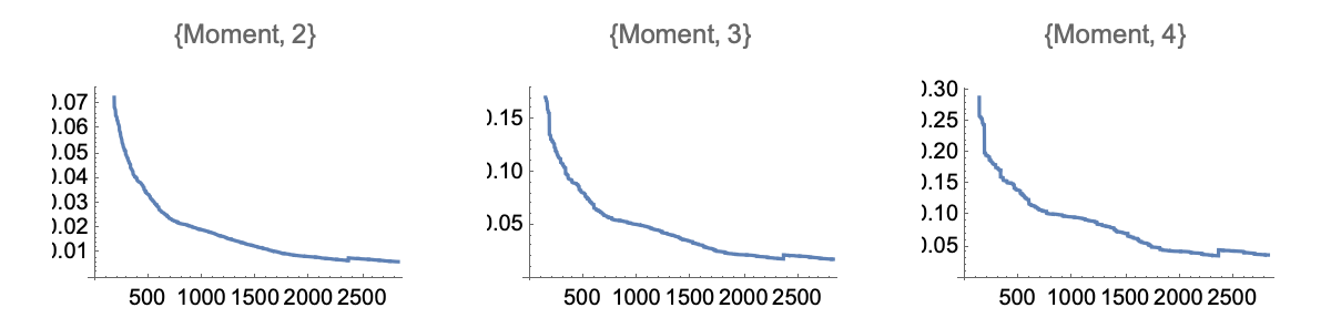
which allows us to obtain p-values below, using \(m=714\) observations (and using the leading order $O(.)$:

Such low p-values exclude any controversy as to their effectiveness cite{taleb2016meta}.
We can also compare rolling correlations using a Monte Carlo for the null with practically the same results (given the exceedingly low p-values). We simulate \(\Delta_{n,m}^o\) with overlapping observations:
\(\Delta_{n,m}^o= \frac{1}{m} \sum_{i=1}^{m-n-1} \rho_n^2(i),\)
Rolling windows have the same second moment, but a mildly more compressed distribution since the observations of \(\rho\) over overlapping windows of length \(n\) are autocorrelated (with, we note, an autocorrelation between two observations \(i\) orders apart of \(\approx 1-\frac{1}{n-i}\)). As shown in the figure below for \(n=36\) we get exceedingly low p-values of order \(10^{-17}\).

Ariely.nbThe “Ariely” fake result reveal a probability distribution totally foreign to psychologists
From @infseriesbot, prove the identity: \(\gamma_n = \displaystyle\int_1^\infty \frac{\{x\}}{x^2} (n-\log(x)) \log^{n-1} \, dx \).
We have \(\{x\}=x-i \, \text{for} \, i \leq x \leq i+1\),
so
\(\text{rhs}=\displaystyle\sum _{i=1}^{\infty } \displaystyle\int_i^{i+1} \frac{(x-i) (n-\log (x)) \log ^{n-1}(x)}{x^2} \, dx,\)
and since \(\displaystyle\int \frac{(x-i) (n-x \log ) \left(x \log ^{n-1}\right)}{x^2} \, dx=\log ^n(x) \left(-\frac{i}{x}-\frac{\log (x)}{n+1}+1\right)\)
\(\displaystyle \int_i^{i+1} \frac{(x-i) (n-\log (x)) \log ^{n-1}(x)}{x^2} \, dx=\frac{(i+1) \log ^{n+1}(i)+(-(i+1) \log (i+1)+n+1) \log ^n(i+1)}{(i+1) (n+1)}\),
allora:
\(\text{rhs}=\underset{T\to \infty }{\text{lim}}\left(\frac{(n-(T+1) \log (T+1)+1) \log ^n(T+1)}{(n+1) (T+1)}+\sum _{i=2}^T \frac{\log ^n(i)}{i}\right)\),
and since \(\frac{\log ^n(T+1) (n-(T+1) \log (T+1)+1)}{(n+1) (T+1)}\overset{T}{\to}\frac{\log ^{n+1}(T)}{n+1}\),
From the series representation of the Stieltjes Gamma function, \(\gamma_n\):
\(\underset{T\to \infty }{\text{lim}}\left(\sum _{i=1}^T \frac{\log ^n i}{i}-\frac{\log ^{n+1}(T)}{n+1}\right)=\gamma _n\)
A maximum entropy alternative to Bayesian methods for the estimation of independent Bernouilli sums.
Let \(X=\{x_1,x_2,\ldots, x_n\}\), where \(x_i \in \{0,1\}\) be a vector representing an n sample of independent Bernouilli distributed random variables \(\sim \mathcal{B}(p)\). We are interested in the estimation of the probability p.
We propose that the probablity that provides the best statistical overview, \(p_m\) (by reflecting the maximum ignorance point) is
\(p_m= 1-I_{\frac{1}{2}}^{-1}(n-m, m+1)\), (1)
where \(m=\sum_i^n x_i \) and \(I_.(.,.)\) is the beta regularized function.
EMPIRICAL: The sample frequency corresponding to the “empirical” distribution \(p_s=\mathbb{E}(\frac{1}{n} \sum_i^n x_i)\), which clearly does not provide information for small samples.
BAYESIAN: The standard Bayesian approach is to start with, for prior, the parametrized Beta Distribution \(p \sim Beta(\alpha,\beta)\), which is not trivial: one is contrained by the fact that matching the mean and variance of the Beta distribution constrains the shape of the prior. Then it becomes convenient that the Beta, being a conjugate prior, updates into the same distribution with new parameters. Allora, with n samples and m realizations:
\(p_b \sim Beta(\alpha+m, \beta+n-m)\) (2)
with mean \(p_b = \frac{\alpha +m}{\alpha +\beta +n}\). We will see below how a low variance beta has too much impact on the result.
Let \(F_p(x)\) be the CDF of the binomial \( \mathcal{B} in(n,p)\). We are interested in \(\{ p: F_p(x)=q \}\) the maximum entropy probability. First let us figure out the target value q.
To get the maximum entropy probability, we need to maximize \(H_q=-\left(\;q \; log(q) +(1-q)\; log (1-q)\right)\). This is a very standard result: taking the first derivative w.r. to q, \(\log (q)+\log (1-q)=0, 0\leq q\leq 1\) and since \(H_q\) is concave to q, we get \(q =\frac{1}{2}\).
Now we must find p by inverting the CDF. Allora for the general case,
\(p= 1-I_{\frac{1}{2}}^{-1}(n-x,x+1)\).
And note that as in the graph below (thanks to comments below by
You have zero probability of making money. But it is a great trade.
One-tailed distributions entangle scale and skewness. When you increase the scale, their asymmetry pushes the mass to the right rather than bulge it in the middle. They also illustrate the difference between probability and expectation as well as the difference between various modes of convergence.
Consider a lognormal \(\mathcal{LN}\) with the following parametrization, \(\mathcal{LN}\left[\mu t-\frac{\sigma ^2 t}{2},\sigma \sqrt{t}\right]\) corresponding to the CDF \(F(K)=\frac{1}{2} \text{erfc}\left(\frac{-\log (K)+\mu t-\frac{\sigma ^2 t}{2}}{\sqrt{2} \sigma \sqrt{t}}\right) \).
The mean \(m= e^{\mu t}\), does not include the parameter \(\sigma\) thanks to the \(-\frac{\sigma ^2}{2} t\) adjustment in the first parameter. But the standard deviation does, as \(STD=e^{\mu t} \sqrt{e^{\sigma ^2 t}-1}\).
When \(\sigma\) goes to \(\infty\), the probability of exceeding any positive \(K\) goes to 0 while the expectation remains invariant. It is because it masses like a Dirac stick at \(0\) with an infinitesimal mass at infinity which gives it a constant expectation. For the lognormal belongs to the log-location-scale family.
\(\underset{\sigma \to \infty }{\text{lim}} F(K)= 1\)
Option traders experience an even worse paradox, see my Dynamic Hedging. As the volatility increases, the delta of the call goes to 1 while the probability of exceeding the strike, any strike, goes to \(0\).
More generally, a \(\mathcal{LN}[a,b]\) has for mean, STD, and CDF \(e^{a+\frac{b^2}{2}},\sqrt{e^{b^2}-1} e^{a+\frac{b^2}{2}},\frac{1}{2} \text{erfc}\left(\frac{a-\log (K)}{\sqrt{2} b}\right)\) respectively. We can find a parametrization producing weird behavior in time as \(t \to \infty\).
Thanks: Micah Warren who presented a similar paradox on Twitter.
The main paper Bitcoin, Currencies and Fragility is updated here .
The supplementary material is updated here
www.fooledbyrandomness.com/BTC-QF-appendix.pdf
BTC-QF-appendix
Prove
\(I= \displaystyle\int_{-\infty }^{\infty}\sum_{n=0}^{\infty } \frac{\left(-x^2\right)^n }{n!^{2 s}}\; \mathrm{d}x= \pi^{1-s}\).
We can start as follows, by transforming it into a generalized hypergeometric function:
\(I=\displaystyle\int_{-\infty }^{\infty }\, _0F_{2 s-1} (\overbrace{1,1,1,…,1}^{2 s-1 \text{times}}; -x^2)\mathrm{d}x\), since, from the series expansion of the generalized hypergeometric function, \(\, _pF_q\left(a_1,a_p;b_1,b_q;z\right)=\sum_{k=0}^{\infty } \frac{\prod_{j=1}^p \left(a_j\right)_k z^k}{\prod_{j=1}^q k! \left(b_j\right)_k}\), where \((.)_k\) is the Pochhammer symbol \((a)_k=\frac{\Gamma (a+k)}{\Gamma (a)}\).
Now the integrand function does not appear to be convergent numerically, except for \(s= \frac{1}{2}\) where it becomes the Gaussian integral, and the case of \(s=1\) where it becomes a Bessel function. For \(s=\frac{3}{2}\) and \( x=10^{19}\), the integrand takes values of \(10^{1015852872356}\) (serious). Beyond that the computer starts to produce smoke. Yet it eventually converges as there is a closed form solution. It is like saying that it works in theory but not in practice!

For, it turns out, under the restriction that \(2 s\in \mathbb{Z}_{>\, 0}\), we can use the following result:
\(\int_0^{\infty } t^{\alpha -1} _pF_q \left(a_1,\ldots ,a_p;b_1,\ldots ,b_q;-t\right) \, dt=\frac{\Gamma (\alpha ) \prod {k=1}^p \Gamma \left(a_k-\alpha \right)}{\left(\prod {k=1}^p \Gamma \left(a_k\right)\right) \prod {k=1}^q \Gamma \left(b_k-\alpha \right)}\)
Allora, we can substitute \(x=\sqrt(u)\), and with \(\alpha =\frac{1}{2},p=0,b_k=1,q=2 s-1\), given that \(\Gamma(\frac{1}{2})=\sqrt(\pi)\),
\(I=\frac{\sqrt{\pi }}{\prod _{k=1}^{2 s-1} \sqrt{\pi }}=\pi ^{1-s}\).
So either the integrand eventually converges, or I am doing something wrong, or both. Perhaps neither.
Background: We’ve discussed blood pressure recently with the error of mistaking the average ratio of systolic over diastolic for the ratio of the average of systolic over diastolic. I thought that a natural distribution would be the gamma and cousins, but, using the Framingham data, it turns out that the lognormal works better. For one-tailed distribution, we do not have a lot of choise in handling higher dimensional vectors. There is some literature on the multivariate gamma but it is neither computationally convenient nor a particular good fit.
Well, it turns out that the Lognormal has some powerful properties. I’ve shown in a paper (now a chapter in The Statistical Consequences of Fat Tails) that, under some parametrization (high variance), it can be nearly as “fat-tailed” as the Cauchy. And, under low variance, it can be as tame as the Gaussian. These academic disputes on whether the data is lognormally or power law distributed are totally useless. Here we realize that by using the method of dual distribution, explained below, we can handle matrices rather easily. Simply, if \(Y_1, Y_2, \ldots Y_n\) are jointly lognormally distributed with a covariance matrix \(\Sigma_L\), then \(\log(Y_1), \log(Y_2), \ldots \log(Y_n)\) are normally distributed with a matrix \(\Sigma_N\). As to the transformation \(\Sigma_L \to \Sigma_N\), we will see the operation below.
Let \(X_1=x_{1,1},\ldots,x_{1,n}, X_2= x_{2,1},\dots x_{2,n}\) be joint distributed lognormal variables with means \(\left(e^{\mu _1+\frac{\sigma _1^2}{2}}, e^{\mu _2+\frac{\sigma _2^2}{2}}\right)\) and a covariance matrix
\(\Sigma_L=\left(\begin{array}{cc}\left(e^{\sigma _1^2}-1\right) e^{2 \mu _1+\sigma _1^2}&e^{\mu _1+\mu _2+\frac{\sigma _1^2}{2}+\frac{\sigma _2^2}{2}}\left(e^{\rho \sigma _1 \sigma _2}-1\right)\\ e^{\mu _1+\mu _2+\frac{\sigma _1^2}{2}+\frac{\sigma _2^2}{2}}\left(e^{\rho \sigma _1 \sigma _2}-1\right)&\left(e^{\sigma _2^2}-1\right) e^{2 \mu _2+\sigma _2^2}\end{array}\right)\)
allora \(\log(x_{1,1}),\ldots, \log(x_{1,n}), \log(x_{2,1}),\dots \log(x_{2,n})\) follow a normal distribution with means \((\mu_1, \mu_2)\) and covariance matrix
\(\Sigma_N=\left(\begin{array}{cc}\sigma _1^2&\rho \sigma _1 \sigma _2 \\ \rho \sigma _1 \sigma _2&\sigma _2^2 \\ \end{array}\right)\)
So we can fit one from the other. The pdf for the joint distribution for the lognormal variables becomes:

\(f(x_1,x_2)= \frac{\exp \left(\frac{-2 \rho \sigma _2 \sigma _1 \left(\log \left(x_1\right)-\mu _1\right) \left(\log \left(x_2\right)-\mu _2\right)+\sigma _1^2 \left(\log \left(x_2\right)-\mu _2\right){}^2+\sigma _2^2 \left(\log \left(x_1\right)-\mu _1\right){}^2}{2 \left(\rho ^2-1\right) \sigma _1^2 \sigma _2^2}\right)}{2 \pi x_1 x_2 \sqrt{-\left(\left(\rho ^2-1\right) \sigma _1^2 \sigma _2^2\right)}}\)
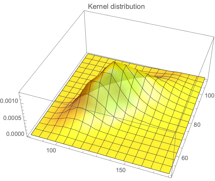
We have the data from the Framingham database for, using \(X_1\) for the systolic and \(X_2\) for the diastolic, with \(n=4040, Y_1= \log(X_1), Y_2=\log(X_2): {\mu_1=4.87,\mu_2=4.40, \sigma_1=0.1575, \sigma_2=0.141, \rho= 0.7814}\), which maps to: \({m_1=132.35, m_2= 82.89, s_1= 22.03, s_2=11.91}\).
